We show the generality and intuition of Lagrangian optimization by showing an example that is well outside the scope of image coding or even engineering. This will hopefully highlight the general applicability of this class of techniques even to general problems involving resource allocation that we are faced with in our day-to-day lives.
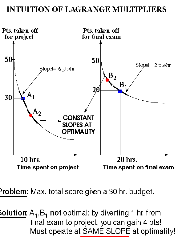
Let us take the example of Bob Smart, a physics freshman at a U.S. 4-year college. It is three weeks before Finals Week, and Bob, like all motivated freshmen, is taking 5 demanding courses, one of which is Physics 101. Bob wakes up to the realization that his grade for the course will be based on (i) a term project that he has not started on yet, and (ii) a Final exam. Each of these two components is worth 50% of the grade for the course. As Bob has spent a few more hours on his extra-curricular activities than he probably should have, and he has to devote a considerable amount of his time to the other courses as well, he realizes that he has to budget his study time for Physics very carefully. Suppose he is able to project his expected performance on both the project and the final exam based on how much time he devotes to them, and further he can quantify them using the curves shown in figures shown below, which measure his expected deviation from perfection (50 points for each component) versus the amount of time spent on the component. After carefully surveying his situation, Bob realizes that he can spare a maximum of 30 hours total between both the project and the final exam. The question is: how does he allocate his time optimally in order to maximize his score in the course?
One option would be for him to devote 10 hours to the project (Bob was never big on projects!) and 20 hours to studying for the final exam. This would amount to operating on Points and in figure below. Based on the tradeoff that models Bob's propensity with respect to both the project and the exam, this would result in an expected score of 20 (or a deviation of 30 from 50) on the project (point ) and a score of 30 on the final exam (point ) for a net of 50 points. This does not bode well for Bob but can he make better use of his time? The answer lies in the slopes of the tradeoff curves that characterize both the project and the final exam. Operating point has an absolute slope of 6 points/hour, while operating point has a slope of only 2 points/hour. Clearly, Bob could help his cause by diverting one hour from the final exam to the project: this would increase his performance by 4 points! It is clear that he should keep stealing time from the final exam study time and spending it on the term project until he derives the same marginal return for the next hour, minute or second that he spends on either activity. This is exactly the operating points and on the curves which live on the same slope of the tradeoff characteristics.
This is exactly the constant slope paradigm alluded to in the body of the text. In a compression application, the tradeoffs involve rate and distortion rather than scores on exams and studying time, but the principles are the same. An important point to be emphasized in this example is that the constant-slope condition holds only under the constraint that the rate-distortion (or equivalent tradeoff) curves are independent. In our example above, this means that we assume that the final exam curve is independent of the project curve, something that may or may not be true in reality. If the amount of time spent on the project influences Bob Smart's preparedness for the final exam, then we have a case of ``dependent coding'' for the compression analogue.
Figure:
Illustration of Lagrangian optimization.
To, demonstrate the above idea we have developed two JAVA applets. The idea behind the the applets is that there are (N) blocks of information and (Q) quantizers. For, simplicity we have assumed that the rate goes from 1 to Q. The data has been generated using a scalar quantizer and random input. The first applet is an example where we fix the number of blocks to 4, the number of quantizer to 3 and the rate-constraint that the algorithm has to achieve is 6. We explain the steps of the Lagrangian Multiplier algorithm as the applet works it way towards optimality.
In the second applet, the user can choose the number of block, number of quantizers and the Rate constraint(Rc) he wants to achieve. Some of the data is from scalar quantizer and some from a random non-increasing data set.
If, the applet window does not fit in your screen, please try this lower version of the above applets. If, you continue to have problems please let us know.
Rate Distortion Theory Homepage